Max Hernandez

Laberinto - Ejemplo de Canvas en HTML5
Mostrando las entradas con la etiqueta Teoría de la información y métodos de codificación. Mostrar todas las entradas

miércoles, 8 de mayo de 2013

Homework 5: Error correction

For this week's class information theory and coding methods, we were given the task of implementing a block code for a binary transmission channel that is able to find and correct errors in the transmission. The algorithm we chose is to calculate the Hamming code and this publication will serve as a report for this task.

The Hamming Code


[image obtained from:"http://thebestschools.org/wp-content/uploads/2011/08/hamming_cat.jpg"]
Hamming code is an algorithm created by Dr. Richard Hamming a remarkable American mathematician who worked in many applications in computer science and telecommunications. This method adds code to a data or group of data to detect bit errors when the data is stored or transmitted from one computer to another.

Parity bits
The algorithm use to detect errors parity bits. The parity bits are bits that are added to data to indicate whether the number of bits that appear in positions indicated are odd or even, in the case of the algorithm Hamming if the number of bits is odd, the parity bit is set to 1 in case of pair has value 0.

Example:
Given this word as input:
01010
And by adding a parity bit at the beginning of the chain to check all bits in the same word would be:
[0]01010
The parity bit in square brackets, is zero because the number of ones in the data is two on two is an even number.

Cheking errors
Since the parity bit is the amount of numbers on the chain, if a bit of the original word does change then the number of bits it will be odd and this is not consistent with the parity bit.

example:
Our word with parity bit is:
001010
If a bit change in the fourth position:
001110
To check if the word change, we just have to recalculate the parity bit for the chain, which in this case is 1, which does not match the parity bit of the string is zero.

Building the Hamming code
Given a word we have to create a new word, ensuring that they have parity bits in positions that are powers of two: 1, 2, 4, 8, 16, etc. The bits of the original word are put in the spaces that are between parity bits.

Example:
for the word:
01010
Parity bits are added in power of two positions with this output:
__1_101_0
 
Now depending of their position to each parity bit position each parity bit have assigned different bits, if the parity bit is in position 1 (counting positions from 1 and not from 0) it has assign itself a bit and skipped a bit, if it is in position 2 are checked two and skip two positions.
Calculating each bit of parity with their respective positions, we have the following string:

010010100

Find bit with error
After taking the Hamming code we can check if one of the bits of the word changed by recalculate all parity bits in the word to recalculate the Hamming code, if the parity bits are different then a bit has been altered and the sum of the positions of parity bits that differ is the value of the error position. Example:

Taking the Hamming code $010010100$ y modifying a bit $011010100$ we can know which bit has change by calculating again the parity bits of this word:
__1_101_0

101010100

Know to know if there is a change in the words we apply an exor:
011010100
101010100
---------
110000000


 We realize that there is a change in the parity bits in positions 1 and 2, adding these positions $1 +2 =  3$ we know that the modified bit is to position 3 and we can change it in the first modified Hamming code for the Hamming code generated in the above example.
011010100$ --> $010010100$ = $010010100 


Applications
Error correction is very important in many areas of computing to name some of the applications:

  • Internet for sending packages commonly adds a checksum value to verify the contents and minimize processing costs.
  • Travel deep into space, due to the difficulty that send messages over long distances with out noise in space.
  • Data saved, because eventually it would have data errors.
  • Satellite broadcasting, cause it helps increase the data delivery ratio.

My implementation
My implementation of this algorithm was build in Python programming language and i used gnuplot for graphs. The implementation was done on a transmission code to simulate a binary channel for the task one done in this class.
 
Code


Result
To show the implementation in the first part as input it gives as input the same string used in the previous example, and in the second part it also generate random words and simulates the sending of a channel with little chance of error in the words, then shows the number of errors found and these few were arranged.

max@max-laptop:~/Dropbox/teoria_informacion/homework5$ python hamming.py 
Example with one error
Original Word: 01010
Recived word:  011010100
Checked word:  010010100

generating 250 words...
Words without errors: 221
Fixed words: 2
Not fixed words: 27

Experiment
As an experiment i wanted to know how efficient the algorithm correcting errors, for which we used the simulator to transmit words and then count how many words are corrected, increasing the ratio of errors for the first experiment. The second experiment was the same as above but this time you increase the amount of bits per Hamming code.

Resut:

Increasing the ratio of errors

Increasing the number of bit per word

Conclusions
Since my implementation is capable of correcting single bit, can be inefficient when the number of errors in a channel is very high. My theory was that the algorithm been affect by chain length too, but as can be seen in the graph it is not determinant for the algorithm.
I would use this implementation just in channels with few errors in which the number of bits per Hamming code is not very big.

Referencias:
http://users.cs.fiu.edu/~downeyt/cop3402/hamming.html
http://whatis.techtarget.com/definition/Hamming-code
http://es.wikipedia.org

miércoles, 24 de abril de 2013

Homework 4: adaptive coding


For this week's class information theory and coding methods, we were given the task of thinking and to code a Huffman algorithm version made ​​of the last implementation made for the last class (link) to be able to function, taking as input the text online, this is getting character by character without actually knowing the frequency of all characters in the text.

My implementation of adaptative Huffman algorithm
The Huffman algorithm is a coding or compression algorithm, which takes a group of characters and their frequencies and generates Huffman codes which are used to perform compression.
The algorithm works by using frequencies of each character to build a binary tree, the path made from the root of the tree is the Huffman code character associated with the character and is used for compression.
The algorithm works on the premise that the more frequently characters should have shorter Huffman codes.
To ensure that the most frequent characters are shorter, We create the tree gathering the leaves are less frequently as children of a new node, this continue until it is a single root node for all characters.

In order to function adaptively, what i added is very simple, before you can compress character by character, the program stored in a variable buffer indicated amount of characters, this is used to calculate an initial tree Huffman coding, only that it add a node with zero frequency as a character, the character which is given the name of 'Joker', it has low frequency and represents the characters that have not appeared yet since these also have low frequency.


Now once we have an initial tree we can encode character by character as they come, the idea is that if you get a character that is not in the tree, add two children to the node "Joker", the new character and another "Joker" node, if we find another character that is not in the tree we will add this in the same way in the last "Joker" node.

In this example draws only the nodes that are added, the final Huffman code gather all nodes "Joker for convenience but serves to explain how adding nodes that have not yet appeared. the added nodes are" Y "and" U ".


Code


Results
To display a graphical results, this graphs are made similar to those of the non-adaptive Huffman task. As initial buffer size chosen 10% of the input text, input texts length vary, red lines are the distribution of letters in Spanish distribution, and the green uniform distribution, these distributions to show Huffman switching between Normal and my implementation of adaptive Huffman.

 The compression ratio estimated from the data compresed split between original data:
Time data encoding of the complete characters:
Time data decoding of the complete characters:

Size of the data obtained:

Suggestions of improvement
My implementation is very simple but I think it could be improved by:

  • Predefined frequencies:Choosing input character frequencies knowing what kind of text is, for example if it is a common text in Spanish there are many frequency tables, as input would receive the characters more frequent in that kind of text.
     
  • Adaptive node adding:
    Seeking a way to accommodate in a adaptive way nodes which are not found in the tree.

References:

http://elisa.dyndns-web.com/~elisa/teaching/comp/info/adaptive.pdf

jueves, 11 de abril de 2013

Huffman encoding algorithm

For this week's class theory of information we were given the task of building an implementation of the Huffman compression algorithm, this publication will serve as a way to report for the task.

Huffman compression algorithm


The Huffman algorithm is a coding or compression algorithm, which takes a group of characters and their frequencies and generates Huffman codes which are used to perform compression.
The algorithm works by using frequencies of each character to build a binary tree, the path made from the root of the tree is the Huffman code character associated with the character and is used for compression.
The algorithm works on the premise that the more frequently characters should have shorter Huffman codes.
To ensure that the most frequent characters are shorter, We create the tree gathering the leaves are less frequently as children of a new node, this continue until it is a single root node for all characters.

An example and an explanation of the method that helped me to understand the workings of the algorithm is in the following video on the channel www.youtube.com "soguw".

To unzip the file, I use a code implementation that used the tree and data bits, bit by bit is traversed the encoded text and each iteration moves through the tree according to bits of the encoded text. It runs from the root, until a final leave, the character of the leave is added to the file decrypted and we get back to the root, go finish it until the bits of the encoded file is traversed.
Code


program running

To demonstrate the program, this running will show the output for text "Huffman", the output of the program was:
max@juan-laptop:~/Dropbox/teoria_informacion/homework3$ python huffman.py

Encoding...

Encoding dictionary: {'a': '100', 'f': '01', 'H': '101', 'm': '110', 'n': '111', 'u': '00', 'root': ''}

Original text: Huffman

Encoded text: 101000101110100111

Compression ratio (compressed / original): 0.0128571428571

Decoding...

Original text: 101000101110100111

Decoded text: Huffman


And the program generated the following tree:


Testing
Now to test the algorithm did some graphs showing various steps of the run of the program, shown in red runs the program on a regular character, these were obtained from the common frequency of occurrence of certain characters in Spanish texts. Green is shown in the worst case, that is one in which the frequency is the same for all characters.

This shows the compression time in seconds, the red line shows a typical case and worst case green, time running time increase en normal case because it need more calculations to find the less frequency nodes, but it is good because if the difference between frequencies increase the compression works better:
This shows the decompression times in seconds:
The amount of memory used for compression:
This shows the compression ratio is the approximate amount of memory of the compressed file divided by the weight of the original file.
As you can see the time to compress and decompress increases for typical cases, but the memory used and clearly the compression ratio decreases.

References:
http://es.wikipedia.org/wiki/Algoritmo_de_Huffman
http://www.cprogramming.com/tutorial/computersciencetheory/huffman.html

jueves, 21 de febrero de 2013

Homework 2: String matching

Hi,this week on information theory and coding methods we are studying algorithms of string matching, so the homework for this week is to implement a program that do string matching, using the Boyer-Moore and Knuth-Morris-Pratt. So this post servers as report of the homework mentioned.

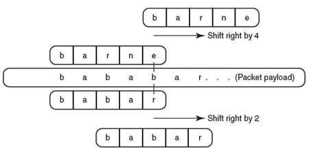
Boyer-Moore algorithm

This algorithm works checking the pattern from left to right, it is considered on of the most efficient of this area.

[Imagen obtenida de:"http://cdn.ttgtmedia.com/digitalguide/images/Misc/netseckia_3.gif"]

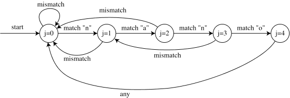
Knuth-Morris-Pratt
This algorithm uses information based on previous failures, using the information to find the very word itself contains to determine which might be the next existence, without having to analyze more than 1 time characters in the search string with.


[imagen obtenida de:"http://www.ics.uci.edu/~eppstein/161/kmp.gif"]
Program code

[]

The program running:
[
max@juan-laptop:~/Desktop/octavo_semestre/teoria_info/homework2$ python homework2.py 
Boyer-Moore
String: 'anita lava la tina'
Pattern: lava
Position: 6

Knuth-Morris-Pratt
String: 'anita lava la tina'
Pattern: lava
Position: 6

012345678901234567
anita lava la tina
]

Time analisys on the algorithms running
For analysis propose, i writed a códe that, measure the running time o the both algorithm using the same text, and pattern, but with diferent length of the twice variables. 

The analisys works generating frst a pattern with aleatory characters, then the code put the pattern in the text, and add other aleatoy characters to fill the text.

This is the gnuplot code, i used a 3d graph because my goal is to show diferences betwen the two algorithms.

set terminal postscript eps enhanced color font 'Helvetica,40'
set output 'introduction.eps'
set size 4, 4
set xlabel 'Pattern length'
set ylabel 'Text length'
set zlabel 'time running'
set logscale
splot "time_test.dat" using 1:2:3 with dots title 'Boyer-Moore' , 'time_test.dat' using 1:2:4 with dots title 'Knuth-Morris-Pratt';
] 
Now the graphic shows in x and y axis the length of the pattern and text, the z-axis shows the time-running used to find the pattern in the text. is used the logscale to show more clearly the difference in the running-time. 


Referencias:
http://www.wikipedia.org/ 

miércoles, 6 de febrero de 2013

Homework 1: Noissy channel simulation

This week on information theory class we discuss the channel transmission systems topic way to connect a transmitter to a receiver in some information transferring. The homework for this week is to build a binary symmetric channel simulation, them make data transmission by the channel and then make some analysis of the simulation output.

Binary symmetric channel simulation
The simulation works this way:
The program receives as parameters the 0 symbol frequency in a word, and a matrix describing the probability of a Symbol to become in another on the transmission, our symbols are just "0" and "1" because we are working with a binary alphabet.

First we simulate a message, for this propose this is done using the "generate_word" method that receives as input the word length and using Bernoulli trials with the 0 frequency obtained as parameter, simulate symbol by
symbol of the word.

Next thing to do is to send the message, this is done with the method "word_transmission" walking symbol by symbol in the word and applying a Bernoulli trial to each symbol, using the matrix of change in a transmission received as a parameter.


https://github.com/MaxHernandez/teoria_informacion

Simulation output analysis
For the analysis part i build a bash script that execute the last python script
and make graphs with the output value, on the graph the Y axis shows the percent of success sending and the X shows the length of the word sent.


https://github.com/MaxHernandez/teoria_informacion

With 90% of frequency occurrence of "0" symbols:
X axis shows the length of the word sent
Y axis shows the percent of success sending a message
With 50% of frequency occurrence of "0" symbols:
X axis shows the length of the word sent
Y axis shows the percent of success sending a message

With 70% of frequency occurrence of "0" symbols:
X axis shows the length of the word sent
Y axis shows the percent of success sending a message

Estimating the asymptotic probability
I could not estimate the accurate asymptotic probability of the output values, but i arrive to the conclusion using the last graphs that the output behaves as an exponential function with negative input $exp(-xC)$ and increasing the probabilityity of success of no change of symbols in transmissions must increase the function constant input $C$.

This is the last graph, but adding the $exp(-x)$ function, as we look the output behaves as and exponential function but i couldn't accurate the function.


References:
http://en.wikipedia.org/wiki/Binary_symmetric_channel
http://elisa.dyndns-web.com/~elisa/teaching/comp/info/channel.pdf